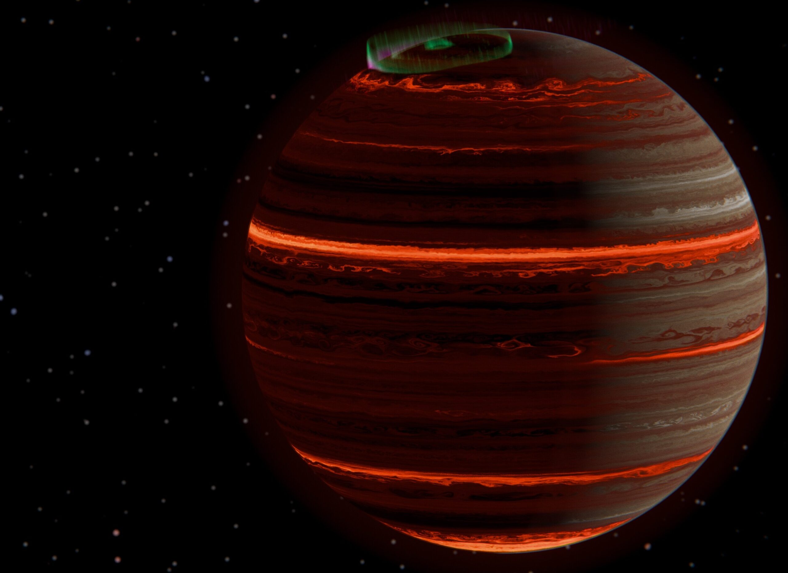
As SIMP 0136 rotates, its infrared spectrum moves through a remarkably simple pattern: despite thousands of individual wavelength measurements changing over time, most of the detectable coherent variability can be described by just two dominant patterns. One is associated with changes in the atmosphere’s thermal structure, while the other is linked to the vertical structure of its clouds. Together, they produce spectra that behave like changing mixtures of three distinct atmospheric states rotating into and out of view.
SIMP J013656.5+093347.3, usually shortened to SIMP 0136, is a young T2.5 brown dwarf near the planetary-mass boundary. The object has an effective temperature of about 1,098 ± 6 kelvins and rotates rapidly, completing a rotation in 2.41 ± 0.08 hours. Previous observations had already shown that its brightness changes as it rotates, with wavelength-dependent variations suggesting that different layers of its atmosphere do not behave in exactly the same way.
The new analysis uses a continuous sequence of observations from the James Webb Space Telescope’s NIRSpec instrument. The observations covered roughly 0.6 to 5.3 micrometers originally, although the analysis trimmed the usable range to 0.9 to 5.3 micrometers because the signal-to-noise ratio fell below the adopted threshold at shorter wavelengths. Taken on July 23, 2023, the sequence lasted 2.9 hours and contained 5,726 individual integrations, giving the researchers a view spanning about 1.2 rotations.
To make the spectra suitable for comparison, the researchers processed each integration individually, accounting for changes in the spectral trace and other time-dependent instrumental effects. They then combined the data into groups of 20 integrations, corresponding to 36.6-second intervals. That produced 287 spectra spread evenly across the observation, with a median signal-to-noise ratio of 73 after the wavelength cuts.
The central question was not simply how much SIMP 0136 brightens and dims. It was whether the complicated wavelength-by-wavelength changes could be reduced to a small number of underlying patterns, and whether those patterns could be connected to physical changes in the atmosphere.
For that, the researchers turned to principal component analysis, or PCA.
PCA looks for groups of wavelengths that change together. Instead of treating every wavelength as an independent variable, it rotates the mathematical description of the data so that the new axes point along the directions where the spectra vary most strongly. Each principal component is therefore a characteristic pattern of spectral change accompanied by a time-dependent score showing how strongly that pattern is present.
Importantly, the principal components are not themselves photographs or spectra of individual atmospheric regions. They describe patterns in how the observed spectrum changes. The physical interpretation comes only after those patterns are compared with atmospheric models and other evidence.
Two components account for the coherent signal
The researchers used a noise-weighted version of PCA because some wavelengths have substantially larger uncertainties than others. Each wavelength was scaled according to its characteristic uncertainty before the decomposition, reducing the influence of noisy channels and allowing coherent spectral changes to dominate the analysis.
The result was strikingly low-dimensional.
The first two principal components accounted for 79% of the total variance in the dataset. But that number alone does not mean that 79% of the variance was astrophysical, because photon and detector noise also contribute to the total variance.
The researchers therefore tested what remained after removing the first two components. The first three components had RMS variability amplitudes of 0.43%, 0.29% and 0.07%, respectively. After the first two were removed, the remaining spectra had an RMS scatter of 0.36%, essentially matching the propagated noise floor of 0.37%. The reduced chi-squared was 0.97. The median lag-1 correlation of the noise-normalized residuals also fell from 0.74 before the subtraction to 0.08 afterward.
In other words, the researchers found no measurable excess of coherent spectroscopic variability beyond those first two components.
The time-dependent scores of both components also showed near-periodic behavior consistent with SIMP 0136’s measured rotation period. That indicated that the patterns were tied to the object’s changing view as it spun.
The two components were not simply two separate pieces of the spectrum. Both contain structure across overlapping wavelength regions, because PCA identifies independent patterns of covariance across the full spectrum rather than assigning each component to a particular wavelength interval.
This provided the first major simplification: a spectrum containing hundreds of wavelength channels could be followed through time using two dominant axes.
The next question was what those axes represented physically.
One axis follows thermal changes, the other follows clouds
The researchers projected a grid of Sonora Diamondback atmospheric models into the same two-dimensional principal-component plane occupied by the observations. The models vary properties including effective temperature, metallicity and cloud sedimentation efficiency.
The sedimentation parameter, known as fsed, describes the balance between turbulent mixing that keeps cloud particles aloft and gravitational settling that pulls them downward. Lower fsed corresponds to thicker, more vertically extended clouds, while higher fsed corresponds to thinner, more settled clouds.
The model grid revealed a clear separation in the observed PCA plane. Changes in effective temperature ran mainly along the first principal-component direction. Changes in fsed ran mainly along the second. Metallicities did not show an obvious corresponding trend.
The model comparison provided another quantitative check. The first observed principal component could reconstruct 35.9% of the variance across the entire model grid. The first two together reconstructed 79.9%. Adding a third component raised that only to 80.2%.
That agreement does not mean that SIMP 0136 literally changes its intrinsic effective temperature as it rotates. The authors explicitly interpret the temperature-like PCA direction as a proxy for changes in the atmosphere’s thermal profile and the distribution of emerging radiation, rather than a change in the object’s internal energy.
For a convective brown dwarf, the researchers note, the deep interior is not expected to change substantially over a few-hour rotation. Instead, spatial differences in atmospheric structure can alter how much radiation emerges from different regions. As the object turns, those regions move into and out of view, changing the disk-integrated spectrum.
The cloud interpretation is similarly qualified. The PCA direction aligns with the fsed direction in the self-consistent model grid, but the two axes are not expected to coincide perfectly. PCA identifies statistically orthogonal directions of maximum covariance, while temperature and cloud properties in atmospheric models are physically coupled. Changing cloud opacity can itself alter the temperature structure and the atmospheric layers from which radiation emerges.
The researchers therefore describe PC1 as primarily temperature-like variability and PC2 as variability associated with cloud vertical structure.
The spectrum moves among three atmospheric states
Once the observations were reduced to two dimensions, another pattern became visible.
A two-dimensional dataset can be enclosed by a triangle whose three vertices represent the minimum set of extreme states needed to contain all the observations. The researchers used this geometric construction to define three spectral “endmembers.”
These are not pure spectra from three isolated spots on the brown dwarf. Every observation is disk-integrated, meaning it combines radiation from many regions at once. The endmembers are conservative estimates of the most extreme atmospheric states actually sampled during this particular observation. The true physical extremes could lie outside the observed range.
The three states occupy different parts of the temperature-cloud sequence.
The first represents a relatively hotter state with comparatively thinner clouds. The second is also associated with relatively thin clouds but at a lower temperature. The third has a similarly lower temperature but substantially more vertically extended clouds.
The observed spectra move around this triangular region as SIMP 0136 rotates. In that sense, the changing spectrum can be represented as a shifting mixture of the three endmembers.
The researchers calculated the fractional contribution of each endmember at every time step using barycentric coordinates, which assign three non-negative weights that add up to one. They propagated the measurement uncertainties into these weights with Monte Carlo sampling, drawing 100 realizations for each spectrum.
The resulting contribution curves show the three atmospheric states changing in relative prominence as the object turns.
But those fractions need to be interpreted carefully. Because the endmembers sit at the edge of the observed spectral distribution, their inferred contributions are lower limits on the contributions of the true physical extremes. If a genuinely pure atmospheric state lies outside the observed convex hull, its true peak contribution would be underestimated by the method. The researchers also assume that the relative timing and ordering of the contributions remain meaningful even if those unseen extremes lie beyond the measured range.
That limitation is central to the interpretation. The three endmembers describe the strongest atmospheric states captured during this observation, not permanent, universal components of SIMP 0136.
The molecular bands change with the clouds
The spectral shapes of the three endmembers provide another clue.
The researchers compared their deviations from the average spectrum with absorption cross sections for water, carbon monoxide, methane and carbon dioxide. The first endmember is almost a gray, broadband shift, meaning it becomes brighter without substantially reshaping individual molecular bands.
The other two behave in opposite ways.
Endmember 2 has deeper H₂O, CH₄ and CO absorption features than the average spectrum. Endmember 3 has shallower absorption in those same bands.
The researchers then compared these patterns with simplified model perturbations involving patchy clouds and a localized upper-atmosphere hot spot. The model calculations used representative 15% cloudy and 7.5% hot-spot covering fractions and a hot-spot temperature perturbation near 0.1 bar. The authors caution that these particular models were not designed for low-gravity objects.
Those calculations showed that the 1–2 micrometer flux windows and the 3.7–4.2 micrometer region are sensitive to cloud coverage, while the 2.2–3.6 micrometer range responds to the modeled hot spot.
The observations followed a pattern consistent with changing cloud vertical structure. Endmember 3 has dimmer cloud-sensitive windows while its molecular bands are less pronounced. The authors interpret that combination as consistent with thicker, more vertically extended clouds that move the effective photosphere to lower pressures and partially mask radiation coming from deeper layers where molecular absorption is stronger.
Endmember 2 shows the reverse: brighter flux windows and stronger molecular bands, consistent with thinner, more settled clouds allowing a deeper view into the atmosphere.
The fact that CO₂, H₂O, CH₄ and CO change coherently across the endmembers leads the researchers to suggest that cloud vertical extent, rather than large changes in atmospheric composition, is the primary modulation represented by PC2. That is an interpretation of the combined spectral evidence, not a direct measurement of cloud thickness at a particular location.
The analysis also provides a possible way to understand the apparent phase shifts seen in earlier observations. Instead of requiring a single atmospheric feature to appear at different wavelengths with a simple time delay, the authors propose that different wavelength bands may be responding to different mixtures of the same low-dimensional variability modes. A band more sensitive to the temperature-like PC1 component can therefore have a different light-curve shape from one more sensitive to the cloud-related PC2 component.
Chemistry adds a more complicated signal
The PCA does not eliminate every atmospheric process.
The researchers also projected phase-resolved atmospheric retrievals from an earlier analysis of the same JWST dataset into the PCA plane. Those retrievals produced 24 phase-resolved atmospheric spectra. After correcting for an offset in the retrieved mean spectrum, their sequence closely followed the triangular pattern traced by the observations.
The retrieved effective temperature again followed the PC1 direction.
Carbon dioxide behaved differently. Its retrieved abundance showed a generally inverse relationship with PC1, with higher CO₂ at lower PC1. The relationship was clearest when the model grid indicated thinner clouds and became much weaker when clouds were more vertically extended.
The researchers do not assign that behavior to one confirmed mechanism. They discuss several possibilities.
Changing cloud opacity could alter the pressure level from which radiation emerges, making different rotational phases probe different atmospheric layers even if the bulk CO₂ abundance remains unchanged. Changes in the local temperature-pressure structure could also alter the balance among CO, CH₄ and CO₂. A third possibility is changing vertical mixing, which could move the pressure level at which chemical abundances become chemically “quenched.”
The data do not distinguish cleanly among these possibilities.
Indeed, the retrievals did not show a clear, coherent phase trend in CO or CH₄. The authors say this does not rule out a chemical contribution, but it could mean that any effect is subtle or that retrieval degeneracies limit the sensitivity to those species.
The retrieval analysis also illustrates why different modeling approaches can give somewhat different-looking answers. The Sonora Diamondback models compress cloud behavior largely into the single fsed parameter, making a cloud-related trend easy to see. The retrieval framework instead allows several cloud parameters, including cloud coverage, base pressure, particle size and mass fraction. Those parameters can partially compensate for one another, potentially hiding a coherent change in any individual parameter.
H₂S provides an even less straightforward case. Its retrieved abundance changes significantly in the analysis and shows a distinct, non-monotonic pattern in PCA space, but it does not line up cleanly with either dominant PCA axis. The authors suggest that it could reflect a more localized atmospheric process, while also cautioning that H₂S can act as a compensating parameter in the retrieval because its broad opacity is difficult to distinguish uniquely from effects involving clouds, temperature or other absorbers.
So the two-component PCA picture does not mean that every atmospheric process has been reduced to exactly two physical mechanisms. Rather, the first two components capture the coherent spectroscopic variability detectable in this dataset, while smaller or more degenerate effects can remain within the residuals or within the interpretation of individual retrieved quantities.
Turning spectral mixtures into a map
The changing contribution of each endmember also allowed the researchers to ask where these atmospheric states might be located around the rotating object.
A full rotational unmixing would attempt to recover both the pure atmospheric spectra and their spatial distributions simultaneously. The researchers did not attempt that because the problem is too degenerate for these data. The high spectral and temporal resolution produces many correlated measurements, but those measurements do not provide enough independent spatial information to uniquely reconstruct a detailed surface.
Instead, they fixed the three conservative endmember spectra and solved only for their longitudinal distributions.
The resulting “maps” are therefore one-dimensional brightness patterns showing how strongly each atmospheric state contributes as a function of longitude. They are averaged over latitude and weighted according to which parts of the rotating disk are visible.
For the mapping calculation, the researchers assumed an equator-on viewing geometry and used the standard thermal-emission visibility kernel, which weights the portion of the surface facing the observer according to the cosine of its viewing angle.
They represented each longitudinal pattern with a Fourier series. Because disk integration suppresses many small-scale spatial patterns, the researchers restricted the map to a limited number of harmonics rather than attempting to reconstruct fine surface detail.
They ultimately adopted a maximum harmonic order of four. Increasing the order beyond that produced little improvement in the fit and introduced structure that the visibility kernel could not strongly support. Their appendix shows that the maps produced with two and four harmonics are already quite similar.
The maps consequently contain broad longitudinal sectors rather than sharp spots. Most of their power is in the first two spatial harmonics, producing patterns that are close to sinusoidal.
The three atmospheric states peak at somewhat different rotational phases. The first endmember, associated with the hotter state, has a longitudinal brightness pattern consistent with the temperature-related brightness pattern reported in the earlier retrieval analysis. The second and third endmembers have similar lower temperatures but differ primarily in their cloud structure and peak at different longitudes.
Taken together, the maps describe a photosphere that is longitudinally heterogeneous. Different spectral states rotate into and out of view, producing the observed changes in the spectrum.
But the researchers stress that the amplitude of those mapped contrasts should be regarded as a lower limit. The endmembers themselves are not pure surface spectra, and the true atmospheric extremes could lie outside the observed convex hull. The geometry of which longitudes favor which state is treated as more robust than the absolute strength of the contrasts.
There is also a limitation imposed by the visibility kernel itself. In the exact equator-on case, certain higher-order odd Fourier modes fall into the kernel’s null space and cannot affect the disk-integrated light curve. SIMP 0136 is viewed at an inclination of about 80 degrees rather than exactly 90 degrees, which can leak some power into those otherwise hidden modes, but the authors still avoid treating such fine structure as well constrained.
The same pattern appeared 37 hours earlier
The researchers also compared their NIRSpec results with a separate JWST observation made with NIRISS/SOSS about 37 hours earlier.
The two instruments provided different views of the same object. NIRISS produced 81 spectra over 2.6 hours at a spectral resolving power of about 1,200, while NIRSpec collected roughly 5,600 integrations over 2.9 hours at a resolving power of about 200. NIRISS therefore had finer spectral resolution, while NIRSpec provided much denser time sampling and a broader wavelength range.
When the datasets were brought onto a common wavelength range and resolution, both traced a closed, low-dimensional loop in principal-component space. The NIRSpec sequence formed a smoother and more extended loop because its much denser sampling captured the trajectory more completely. The NIRISS sequence was more sparsely sampled and appeared more compact.
The exact shapes were not identical. The researchers interpret that difference as evidence that the atmospheric state had evolved between the observations, although differences in sampling, normalization and wavelength weighting also affect the detailed geometry.
When PCA was performed separately on the two epochs, the exact eigenspectra differed substantially in some wavelength ranges. Yet projecting the atmospheric models into the two PCA spaces again produced the same basic physical interpretation: the leading component tracked temperature-related changes in emitted flux, while the second emphasized molecular-band and continuum behavior associated with vertical cloud structure.
This led the researchers to describe the result as “same drivers, evolving fingerprints.” The dominant physical axes remain recognizable, but the detailed spectral patterns change as the mean atmospheric state changes.
The comparison also shows why the broad wavelength coverage of JWST matters for the PCA result. When the NIRSpec data were restricted to the 1.1–1.7 micrometer range used in an earlier Hubble Space Telescope analysis, about 92% of the variance collapsed into the first principal component, with the second accounting for less than 1%. The much broader JWST wavelength range includes molecular features such as methane near 3.3 micrometers and carbon dioxide near 4.3 micrometers, allowing additional atmospheric variability to separate into another dominant component.
The earlier Hubble analysis had therefore seen a simpler version of the same low-dimensional behavior. The broader JWST coverage exposes more of the atmosphere and separates the temperature-like and cloud-related signals more clearly.
One rotation is only a snapshot
The PCA analysis gives SIMP 0136 a relatively simple description over the observed rotation, but the comparison between epochs also places a limit on what that snapshot can tell us.
The NIRSpec and NIRISS observations were separated by 33.6 hours, corresponding to 13.9 ± 0.5 rotations. Both retained a low-dimensional structure and the same broad physical interpretation, but the detailed trajectories changed. The researchers interpret that reshaping as evidence that the atmosphere evolves on timescales longer than a single rotation.
That means the three endmembers identified from the NIRSpec observation should not be regarded as permanent atmospheric components. They are the extreme states sampled during one particular rotation. If the object were monitored for additional rotations while its atmosphere evolved, the observed range could expand and the PCA-defined endmembers could change.
The authors also emphasize that their PCA result does not establish a unique detailed map of SIMP 0136. The true pure atmospheric spectra may lie outside the observed convex hull, and allowing such unseen extremes can alter the inferred directions in principal-component space. Likewise, disk integration removes spatial information, preventing the data from uniquely determining fine-scale surface structure.
What the observations do support is a more constrained picture: the detectable coherent spectral variability is low-dimensional, with two dominant patterns, and those patterns are consistent with thermal-profile changes and cloud vertical structure. The changing proportions of three conservative spectral states then provide a way to describe how heterogeneous atmospheric regions rotate through view.
The comparison with the earlier JWST epoch adds another qualification. The dominant modes appear to persist, while their detailed spectral fingerprints evolve. The researchers therefore describe SIMP 0136 as occupying a stable low-dimensional pattern of variability while its precise atmospheric state changes with time. They note that continuous multi-rotation monitoring would be needed to determine how those trajectories themselves evolve.
For the single NIRSpec rotation analyzed here, the result is a compact picture of a rapidly rotating brown dwarf whose changing spectrum is not dominated by a large collection of unrelated variations. Instead, most of the measurable coherent change follows two principal directions. One tracks changes in the atmosphere’s thermal structure. The other tracks changes in the vertical extent of clouds. Those two directions combine into three conservative atmospheric states whose contributions rise and fall at different rotational phases, producing the broad longitudinal patterns recovered from the data.
The study was published in Astronomy & Astrophysics.