Complexity theory is one of the foundational areas of computer science that allows us to analyze and compare algorithms. It helps us understand how efficiently a given algorithm performs, especially as the size of its input grows. Whether designing an algorithm to sort millions of numbers, search through massive datasets, or process large-scale simulations, complexity theory provides a mathematical framework to evaluate how computational resources such as time and memory scale.
At the heart of complexity theory lie three fundamental asymptotic notations: Big O (O), Big Theta (Θ), and Big Omega (Ω). These notations are tools for expressing how an algorithm behaves as its input size becomes very large. They abstract away details like hardware speed or programming language and focus purely on the growth rate of an algorithm’s resource usage.
Understanding these concepts is crucial because efficient algorithms are not just faster—they make the difference between feasible and infeasible computation. An algorithm that takes linear time might complete in seconds, while one that takes exponential time might not finish even in the lifetime of the universe when the input grows large enough.
The Foundation of Complexity Theory
Complexity theory studies how difficult computational problems are and how efficiently they can be solved. Every algorithm consumes resources such as time (the number of operations it performs) and space (the memory it uses). When we talk about time complexity, we are referring to how the running time of an algorithm increases as a function of input size, usually denoted as n.
The exact running time of an algorithm depends on many factors—processor speed, programming language, compiler optimizations, and even the data itself. However, complexity theory abstracts away these machine-specific details to focus on how the algorithm scales fundamentally. For example, if one algorithm requires roughly n² steps to process n elements, while another requires only n log n steps, the second algorithm will always outperform the first for sufficiently large n, regardless of the hardware used.
This abstraction is achieved using asymptotic analysis, a mathematical approach that looks at the limiting behavior of functions as n grows towards infinity. The goal is not to determine exact execution times but to understand the relative growth rates of functions that describe algorithm performance.
Asymptotic Analysis and Growth Rates
In asymptotic analysis, we express the performance of an algorithm in terms of its order of growth. This order captures how quickly the resource usage increases as the input size expands. For instance, an algorithm with a time complexity of n² grows much faster than one with a time complexity of n log n.
To compare these growth rates formally, we use mathematical notations that describe the upper bounds, lower bounds, and tight bounds of these functions. These are expressed using the Big O, Big Omega, and Big Theta symbols.
Before exploring these notations, it is important to understand that the purpose of asymptotic notation is not to give exact counts of operations but to describe the dominant behavior of a function as n becomes large. For small values of n, constants and lower-order terms may dominate, but asymptotically, they become insignificant. For example, in a function like f(n) = 5n² + 3n + 10, the 5n² term dominates as n grows, so we say the function has an order of n².
Big O Notation: The Upper Bound
Big O notation is the most commonly used asymptotic notation in computer science. It describes the upper bound of an algorithm’s growth rate, representing the worst-case scenario. Formally, if we say that f(n) is O(g(n)), it means that f(n) does not grow faster than a constant multiple of g(n) for sufficiently large n.
In mathematical terms,
f(n) = O(g(n)) if there exist positive constants c and n₀ such that for all n ≥ n₀,
f(n) ≤ c × g(n).
This definition captures the idea that beyond some threshold n₀, g(n) serves as an upper bound for f(n), up to a constant factor. The constant c ensures flexibility to accommodate scaling differences, while n₀ specifies the range after which the approximation holds true.
For example, consider an algorithm whose time complexity is given by f(n) = 3n² + 2n + 5. We can say that f(n) = O(n²) because for large values of n, the n² term dominates, and the function never grows faster than a constant multiple of n².
Big O notation is particularly useful for expressing the worst-case performance of an algorithm, which ensures that even in the most unfavorable conditions, the algorithm will not exceed a particular time complexity.
Big Omega (Ω) Notation: The Lower Bound
While Big O gives an upper limit on growth, Big Omega notation provides the lower bound. It describes the best-case scenario for an algorithm or the minimum rate at which the resource usage grows. Formally, f(n) = Ω(g(n)) means that beyond some point n₀, f(n) grows at least as fast as a constant multiple of g(n).
Mathematically,
f(n) = Ω(g(n)) if there exist positive constants c and n₀ such that for all n ≥ n₀,
f(n) ≥ c × g(n).
This means that g(n) serves as a lower bound for f(n), indicating that no matter how efficiently the algorithm performs in practice, its growth rate cannot be better than Ω(g(n)).
For instance, if the time complexity of an algorithm is f(n) = 2n² + 4n + 7, then f(n) = Ω(n²). This is because, asymptotically, the n² term dominates, and the function cannot grow slower than some constant times n².
Big Omega notation is essential when analyzing the minimum possible effort or time an algorithm might require. While less frequently used in casual algorithm analysis compared to Big O, it is critical for understanding theoretical efficiency limits and proving optimality of algorithms.
Big Theta (Θ) Notation: The Tight Bound
Big Theta notation provides a tight bound, meaning it simultaneously gives both an upper and a lower limit on growth. If f(n) = Θ(g(n)), then f(n) grows at the same rate as g(n) asymptotically. In other words, g(n) is both an upper and lower bound for f(n) up to constant factors.
Formally,
f(n) = Θ(g(n)) if there exist positive constants c₁, c₂, and n₀ such that for all n ≥ n₀,
c₁ × g(n) ≤ f(n) ≤ c₂ × g(n).
This definition captures the idea of asymptotic equivalence: f(n) grows neither faster nor slower than g(n) beyond a certain point.
For example, for f(n) = 5n² + 3n + 4, we can say that f(n) = Θ(n²). The quadratic term dominates both the upper and lower bounds, so the function’s growth is tightly bounded by n².
Big Theta notation is particularly valuable when we want to express the exact asymptotic behavior of an algorithm, rather than just upper or lower limits. If an algorithm’s time complexity is Θ(n log n), it means its runtime grows proportionally to n log n in all cases, up to constant factors.
Comparing Big O, Big Omega, and Big Theta
These three notations complement each other in describing different perspectives of algorithm growth. Big O gives a ceiling, Big Omega gives a floor, and Big Theta identifies the exact asymptotic growth rate.
For example, suppose an algorithm has f(n) = 4n² + 3n + 1. We can describe its complexity as:
- O(n²) because the growth never exceeds some constant times n².
- Ω(n²) because the growth is never slower than some constant times n².
- Θ(n²) because n² tightly bounds f(n) from both above and below.
This relationship shows that if f(n) = Θ(g(n)), then it must also be true that f(n) = O(g(n)) and f(n) = Ω(g(n)) simultaneously. However, the reverse is not necessarily true—an algorithm can be O(g(n)) without being Θ(g(n)) if the upper and lower bounds are not equal.
Practical Examples of Asymptotic Notations
Let us consider a few common examples from algorithmic analysis to better understand these notations.
A linear search that scans through an array of n elements one by one has a time complexity of O(n) in the worst case, because in the worst scenario it might need to inspect every element. In the best case, when the element is found immediately, it takes constant time, so it is Ω(1). The average case complexity is still proportional to n, so it is Θ(n) overall.
A binary search, on the other hand, divides the search interval in half at each step. This leads to a time complexity of O(log n), since the number of steps grows logarithmically with input size. In this case, the lower and upper bounds are the same, so the algorithm’s time complexity is Θ(log n).
A bubble sort algorithm requires comparing and swapping adjacent elements repeatedly. In the worst case, when the list is in reverse order, it performs roughly n² comparisons, making it O(n²). In the best case, when the list is already sorted, it can complete in Ω(n) time (a single pass). However, its average case is still Θ(n²), showing that it scales poorly for large inputs.
These examples demonstrate how asymptotic notations give a powerful vocabulary for describing how algorithms behave in different scenarios without depending on machine-specific details.
The Role of Constants and Lower-Order Terms
One of the most important features of asymptotic notation is that it ignores constants and lower-order terms. This is because asymptotic analysis focuses on how functions behave as n becomes very large.
For example, consider two algorithms with the following time complexities:
- f₁(n) = 100n
- f₂(n) = n²
For small input sizes, f₁(n) may take longer due to the large constant factor. However, as n grows, the n² term dominates, and f₂(n) quickly becomes much slower. In Big O notation, constants like 100 are irrelevant, because they do not affect the long-term growth trend. Thus, f₁(n) is O(n) and f₂(n) is O(n²).
This simplification allows us to reason about algorithm efficiency without being distracted by implementation details.
Analyzing Average, Worst, and Best Cases
While Big O notation is often associated with the worst case, algorithms can also be analyzed in terms of their average-case and best-case complexities.
The worst case describes the maximum time or space the algorithm could possibly take, which is essential for guaranteeing performance under any circumstances. The best case indicates the minimum time, corresponding to Big Omega notation. The average case reflects the expected time given random input distributions and often uses Big Theta notation when it matches the overall asymptotic behavior.
For example, quicksort has a best and average case of Θ(n log n) but a worst case of O(n²). Despite its poor worst-case performance, quicksort is widely used because the average case dominates in practice.
Beyond Time Complexity: Space Complexity and Other Resources
While time complexity receives the most attention, space complexity is equally important in many applications. Space complexity measures how much memory an algorithm uses as a function of input size. Just as with time, asymptotic notations apply to space as well.
For instance, an in-place sorting algorithm such as heapsort uses O(1) additional memory, whereas mergesort requires O(n) auxiliary space. In large-scale computations or embedded systems with limited memory, such distinctions are crucial.
Other forms of complexity can also be analyzed asymptotically, such as communication complexity (data transferred between processors), energy complexity (power consumption in computations), and parallel complexity (efficiency across multiple processors). The underlying principles of Big O, Big Theta, and Big Omega remain applicable across these contexts.
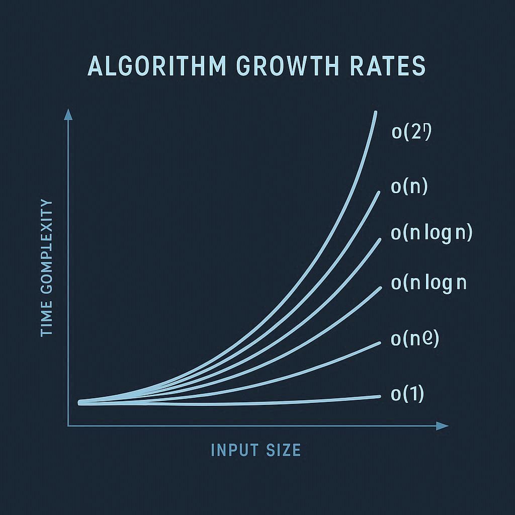
Common Complexity Classes
Algorithms are often categorized into complexity classes based on their asymptotic growth. Constant time algorithms have O(1) complexity, meaning their performance does not depend on input size. Linear time algorithms have O(n) complexity, where running time grows proportionally to input size. Quadratic time algorithms (O(n²)) are common in simple sorting algorithms, while more efficient algorithms like mergesort operate in O(n log n) time.
At the higher end, exponential time algorithms (O(2ⁿ)) and factorial time algorithms (O(n!) ) become infeasible even for modest input sizes. These complexity classes serve as benchmarks for evaluating algorithmic efficiency and determining practical feasibility.
Misconceptions About Big O Notation
A common misconception is that Big O represents the exact running time of an algorithm. In reality, it represents only the upper bound of growth. It also does not indicate whether one algorithm is faster than another for small inputs, since constants and lower-order terms can dominate in such cases.
Another misunderstanding is that Big O always describes the worst case. While it often does in practice, it can also be used to describe upper bounds for average-case behavior when explicitly stated.
Understanding these nuances prevents oversimplified interpretations and ensures accurate communication in algorithm analysis.
The Importance of Complexity Analysis in Real-World Computing
In real-world applications, complexity analysis has profound implications. Search engines, cryptographic algorithms, machine learning models, and data processing pipelines all rely on efficient algorithms to handle massive datasets. An improvement from O(n²) to O(n log n) can reduce processing time from hours to seconds, saving computational resources and energy.
Complexity theory also plays a key role in computational limits. Certain problems, such as the famous P vs NP question, explore whether every problem whose solution can be verified quickly can also be solved quickly. These deep theoretical questions define the boundaries of what is computationally feasible.
The Interplay Between Theory and Practice
Although asymptotic analysis provides powerful insights, practical algorithm performance depends on real-world factors such as constant factors, memory hierarchy, data locality, and hardware parallelism. Thus, empirical testing complements theoretical analysis. An algorithm that is asymptotically optimal may still perform poorly on small inputs or specific architectures if its constants are large.
Therefore, both theoretical and experimental perspectives are necessary. Theoretical complexity gives long-term insight, while benchmarking and profiling ensure that implementations perform well in practice.
Conclusion
Complexity theory, and in particular asymptotic notation, lies at the core of computer science. Big O, Big Theta, and Big Omega notations allow us to describe, compare, and predict the behavior of algorithms in a way that transcends implementation details and machine dependencies. Big O expresses the upper limit, Big Omega the lower limit, and Big Theta the tight bound of an algorithm’s growth rate.
By mastering these concepts, one gains the ability to analyze algorithms rigorously, design efficient computational methods, and understand the inherent limitations of computation itself. Complexity theory not only helps us write better programs—it deepens our understanding of what can be computed efficiently and what cannot. It reveals the mathematical beauty underlying the art of algorithm design and reminds us that in computing, elegance often arises from simplicity, precision, and an awareness of how things scale.