Kinematics is the branch of physics that describes how objects move. It examines an object’s position, distance traveled, displacement, speed, velocity, and acceleration without investigating the forces that cause the motion. From a car traveling down a highway to a ball falling toward the ground, kinematics provides the tools to describe, measure, and predict movement.
By studying how an object’s position changes over time, scientists and engineers can determine where it is, how quickly it is moving, and how its motion changes. These principles are essential in transportation, robotics, astronomy, sports science, and many other fields.
What is kinematics in physics?
Kinematics is the study of motion in terms of measurable quantities, especially position and time. It describes the path an object follows, how far it travels, how fast it moves, and whether its velocity changes.
A key feature of kinematics is that it does not explain why an object moves in a particular way. That question belongs primarily to dynamics, another branch of mechanics that studies the relationship between forces and motion.
Consider a car traveling along a straight road. Kinematics can describe the car’s speed, its direction of travel, how long it takes to reach a destination, and how its velocity changes as it accelerates or brakes. Dynamics, by contrast, investigates the forces from the engine, brakes, road, and air that produce those changes.
Kinematics is therefore a descriptive framework for motion. It provides a mathematical language for understanding movement before examining the physical causes behind it.
Why motion requires a frame of reference
To describe motion accurately, it is necessary to establish a frame of reference. A frame of reference is a coordinate system or viewpoint used to measure an object’s position and movement.
Motion is always described relative to something else. A passenger sitting in a moving car is stationary relative to the car but moving relative to the road. Similarly, a person walking down the aisle of a moving train has one velocity relative to the train and another relative to the ground.
Without a specified reference point, statements about motion can be incomplete or ambiguous.
Physicists often use one-dimensional coordinates to describe motion along a straight line, two-dimensional coordinates for motion across a flat surface, and three-dimensional coordinates for movement through space. The choice depends on the problem being studied.
For example, a ball rolling along a level floor may be adequately described using a single horizontal coordinate. A basketball moving toward a hoop requires at least two coordinates to represent its horizontal and vertical positions.
Choosing an appropriate frame of reference makes motion easier to measure and analyze.
Distance and displacement: Two ways to describe movement
Distance and displacement are closely related, but they describe different aspects of motion.
Distance is the total length of the path an object travels. It is a scalar quantity, meaning it has magnitude but no direction.
Displacement is the change in an object’s position from its starting point to its ending point. It is a vector quantity, meaning it has both magnitude and direction.
Imagine walking 3 miles east and then 3 miles west, returning to your starting point. Your total distance traveled is 6 miles, but your displacement is zero because your final position is the same as your initial position.
This distinction matters whenever an object changes direction. Distance measures the entire journey, while displacement measures the net change in position.
In one-dimensional motion, displacement can be calculated by subtracting the initial position from the final position:
Displacement = Final position − Initial position
Or, using symbols:
Δx = x₂ − x₁
Here, Δx represents the change in position, x₁ is the initial position, and x₂ is the final position.
If a runner begins at the 10-meter mark on a track and finishes at the 50-meter mark, the runner’s displacement is 40 meters in the positive direction. The distance traveled, however, depends on the actual path taken between those positions.
Speed and velocity: How quickly an object moves
Speed and velocity both describe how quickly an object moves, but velocity also accounts for direction.
Speed is the distance traveled per unit of time. Average speed is calculated by dividing the total distance by the total elapsed time.
Average speed = Total distance ÷ Total time
For example, if a car travels 120 miles in 2 hours, its average speed is 60 miles per hour. This does not mean the car maintained that speed throughout the trip. It may have stopped, accelerated, or slowed down along the way.
Velocity describes the rate at which an object’s position changes, including its direction. Average velocity is calculated by dividing displacement by elapsed time.
Average velocity = Displacement ÷ Elapsed time
Suppose a person walks 100 meters east in 50 seconds. The person’s average velocity is 2 meters per second east.
If the person then walks 100 meters west and returns to the starting point, the total distance is 200 meters, but the overall displacement is zero. For the complete trip, the average speed is positive, while the average velocity is zero.
This example demonstrates why speed and velocity cannot always be used interchangeably. Speed describes how much ground an object covers over time, while velocity describes how its position changes over time.
Acceleration: How velocity changes
Acceleration measures how quickly velocity changes with time. An object accelerates when its speed increases, its speed decreases, or its direction changes.
Average acceleration is calculated by dividing the change in velocity by the elapsed time:
a = (v₂ − v₁) ÷ Δt
In this equation, a represents average acceleration, v₁ is the initial velocity, v₂ is the final velocity, and Δt is the elapsed time.
In the International System of Units, acceleration is measured in meters per second squared (m/s²). An acceleration of 3 m/s² means that velocity changes by 3 meters per second during each second, provided the acceleration remains constant.
Consider a car that increases its velocity from 10 m/s to 25 m/s over 5 seconds. Its average acceleration is:
a = (25 − 10) ÷ 5 = 3 m/s²
The car’s velocity increases by an average of 3 m/s each second during that interval.
Acceleration can also be negative, depending on the chosen coordinate direction. For example, a car moving in the positive direction may have negative acceleration when braking. However, negative acceleration does not always mean an object is slowing down. If an object moves in the negative direction and accelerates further in that direction, its speed increases even though its acceleration is negative.
An object can also accelerate without changing its speed. A car traveling around a circular track at a constant speed continually changes direction, so its velocity changes and it experiences acceleration.
The main types of motion studied in kinematics
Kinematics can describe many forms of movement, from objects traveling along straight lines to objects rotating around an axis. Several basic categories help organize these patterns.
Rectilinear motion occurs when an object moves along a straight line. A train traveling along a straight section of track or an elevator moving vertically provides examples. The motion can involve constant velocity, acceleration, or changes in direction.
Curvilinear motion occurs when an object follows a curved path. A car rounding a bend, a thrown ball traveling through the air, and a planet moving along its orbit are examples. Describing this motion often requires tracking changes in both the magnitude and direction of velocity.
Circular motion is a special type of curvilinear motion in which an object travels along a circular path. A rotating fan blade and a point on the rim of a turning wheel illustrate this type of movement. Even at constant speed, an object in circular motion continually changes direction and therefore accelerates.
Rotational motion describes the turning of an object around an axis. A spinning wheel, a rotating door, and a planet turning about its axis are examples. Rotational kinematics uses quantities such as angular position, angular velocity, and angular acceleration to describe how rotation changes over time.
These categories can overlap. A wheel rolling along a road, for example, combines the forward motion of its center with rotation around its axis.
The basic equations of kinematics
For straight-line motion with constant acceleration, a small set of equations connects position, velocity, acceleration, and time. These relationships make it possible to solve many everyday motion problems.
The equations apply when acceleration remains constant over the interval being considered. They do not automatically apply to every moving object, especially when acceleration changes significantly with time.
The first equation relates final velocity to initial velocity and acceleration:
v = v₀ + at
Here, v is final velocity, v₀ is initial velocity, a is constant acceleration, and t is elapsed time.
For example, an object initially moving at 4 m/s accelerates at 2 m/s² for 3 seconds. Its final velocity is:
v = 4 + (2 × 3) = 10 m/s
The second equation calculates displacement using initial velocity, acceleration, and time:
Δx = v₀t + ½at²
This equation accounts for the distance covered by an object that begins with an initial velocity and continues accelerating uniformly.
Using the same example, the displacement is:
Δx = (4 × 3) + ½(2 × 3²) = 21 m
The object travels 21 meters during those 3 seconds.
A third equation relates velocity, acceleration, and displacement without requiring elapsed time:
v² = v₀² + 2aΔx
This relationship is particularly useful when the distance traveled is known but the time is not.
Another useful expression gives displacement for constant acceleration using the average of the initial and final velocities:
Δx = t
This formula works because, under constant acceleration, velocity changes uniformly, making the average velocity equal to the arithmetic mean of the initial and final velocities.
Together, these equations allow physicists and engineers to calculate unknown quantities when the remaining variables are known.
Free fall: Kinematics in action
Free fall is a familiar example of kinematics. Near Earth’s surface, an object in free fall experiences an approximately constant downward acceleration due to gravity when air resistance is negligible.
The magnitude of this acceleration is approximately 9.8 m/s². This means an object’s downward velocity increases by about 9.8 m/s for every second it falls, assuming the idealized conditions remain valid.
Imagine dropping a ball from rest. Its initial vertical velocity is zero. As it falls, gravity increases its downward velocity, and the distance it covers during each successive second becomes greater.
Taking upward as the positive direction, the acceleration due to gravity is approximately −9.8 m/s². The vertical displacement can then be described by:
Δy = v₀t − ½gt²
Here, Δy is the vertical displacement, v₀ is the initial vertical velocity, g is the positive magnitude of gravitational acceleration, and t is elapsed time.
For an object dropped from rest, v₀ equals zero, so the equation simplifies to:
Δy = −½gt²
The negative sign indicates downward displacement under the chosen coordinate convention.
In a vacuum, objects of different masses fall with the same gravitational acceleration at the same location. In everyday conditions, air resistance can cause objects to fall differently. A feather and a metal ball, for instance, may fall at different rates through air because drag affects them differently.
Kinematics describes the resulting motion, while dynamics explains how gravity and air resistance produce it.
Projectile motion: Understanding a ball in flight
Projectile motion occurs when an object is launched into the air and then moves under the influence of gravity, assuming air resistance is negligible.
A thrown baseball, a kicked soccer ball, and water emerging from a fountain are common examples. Their paths are often approximately parabolic because horizontal and vertical motion follow different patterns.
In the idealized model, gravity acts vertically downward. There is no horizontal acceleration, so the horizontal velocity remains constant. Vertically, the object accelerates downward at approximately 9.8 m/s² near Earth’s surface.
These two components can be analyzed separately.
For horizontal motion:
Δx = vₓt
Here, vₓ is the constant horizontal velocity.
For vertical motion:
Δy = vᵧ₀t − ½gt²
Here, vᵧ₀ is the initial vertical velocity.
The combined horizontal and vertical positions determine the projectile’s path. If the object is launched upward at an angle, its vertical velocity decreases as it rises. At the highest point of its trajectory, the vertical velocity is momentarily zero. Gravity continues acting at that point, so the object begins moving downward afterward.
The horizontal velocity does not become zero at the peak in the idealized model. This is why a thrown ball continues traveling forward even as it transitions from rising to falling.
Real projectiles experience air resistance, which can change their trajectories and reduce their horizontal speeds. More detailed kinematic descriptions can incorporate these changes when the motion is measured or modeled over time.
Motion graphs: Reading movement visually
Graphs provide another way to understand kinematics. Instead of describing movement only with equations, physicists can plot position, velocity, or acceleration against time to reveal patterns.
A position-time graph shows how an object’s position changes over time. The slope of the graph represents velocity. A steep slope indicates a large velocity magnitude, while a horizontal segment indicates that the object’s position is not changing.
The sign of the slope indicates direction in a one-dimensional coordinate system. A positive slope means position is increasing, and a negative slope means position is decreasing.
A velocity-time graph shows how velocity changes over time. Its slope represents acceleration. A horizontal segment indicates constant velocity, while a sloping segment indicates changing velocity.
The area between a velocity-time graph and the time axis represents displacement over the corresponding interval. Areas above the axis represent positive displacement, while areas below it represent negative displacement.
An acceleration-time graph shows how acceleration varies over time. The area under this graph represents the change in velocity over the interval.
These relationships make graphs especially useful for interpreting motion sensor data, analyzing vehicle performance, and comparing different movement patterns. A graph can reveal whether motion is steady, accelerating, reversing, or changing in more complex ways.
Kinematics versus dynamics
Kinematics and dynamics are closely connected branches of classical mechanics, but they answer different questions.
Kinematics asks how an object moves. It describes position, velocity, acceleration, and the mathematical relationships among them.
Dynamics asks why an object moves as it does. It examines forces, mass, momentum, and the physical interactions that produce changes in motion.
Consider a car braking at a traffic light. Kinematics describes how the car’s velocity decreases, how long the stopping process takes, and how far the car travels before coming to rest. Dynamics investigates the braking force, tire-road friction, the car’s mass, and other factors that influence deceleration.
The two approaches complement one another. Dynamics can predict the acceleration produced by known forces, and kinematics can use that acceleration to calculate changes in velocity and position.
Neither branch replaces the other. Together, they provide a more complete understanding of physical motion.
Real-world applications of kinematics
Kinematics is used wherever movement must be measured, predicted, or controlled. Its principles are especially valuable in engineering, transportation, sports, robotics, and space exploration.
In automotive engineering, kinematic calculations help determine stopping distances, acceleration times, and vehicle trajectories. Engineers use these relationships when evaluating vehicle handling and designing systems that must respond to changes in speed and direction.
In sports science, motion analysis helps coaches and researchers study running speed, jumping, throwing, and the movements of athletes. By measuring position over time, they can estimate velocity and acceleration and examine how movement changes during a performance.
Robotics relies on kinematics to determine the positions and orientations of moving components. The kinematics of a robotic arm, for example, describes how joint angles determine the location of its end point. This allows a robot to reach a target position without requiring the motion description itself to explain the forces at each joint.
In astronomy and spaceflight, kinematics helps describe the trajectories of planets, satellites, and spacecraft. Scientists and engineers track position and velocity to understand orbital motion and plan changes in a spacecraft’s path. Predicting the effects of gravity and other forces requires dynamics as well, but kinematic descriptions remain essential for representing the resulting trajectories.
Kinematics also appears in ordinary activities such as walking, cycling, throwing a ball, and riding an elevator. Any situation involving measurable changes in position over time can be examined using its principles.
The limitations of classical kinematics
The equations commonly taught in introductory physics describe motion within classical mechanics. They work extremely well for many everyday situations involving objects moving at speeds much lower than the speed of light and at scales where quantum effects are negligible.
However, the simplest equations have specific assumptions. The standard constant-acceleration equations require acceleration to remain constant during the interval being analyzed. If acceleration varies, the motion may require more general mathematical methods, such as calculus or numerical calculations.
Real-world conditions can also complicate a model. Air resistance, changing terrain, moving reference frames, and interactions with other objects may affect motion in ways that a simplified calculation does not capture.
At speeds approaching the speed of light, classical descriptions must be replaced or supplemented by relativistic mechanics. At atomic and subatomic scales, quantum mechanics becomes important because objects cannot always be described adequately using the classical picture of a definite position and trajectory.
These limitations do not make ordinary kinematics unreliable. They show that scientific models are designed for particular conditions and that more advanced descriptions are needed when those conditions no longer apply.
Kinematics provides a foundational way to understand motion by connecting position, time, distance, displacement, velocity, and acceleration. Its equations and graphs turn movement into something that can be measured and predicted, whether the subject is a falling ball, a speeding car, a rotating wheel, or a spacecraft traveling through space. By describing how objects move before investigating why they move, kinematics establishes one of the essential foundations of physics.